
Cardiovascular
Machine learning analysis and risk prediction of weather-sensitive mortality related to cardiovascular disease during summer in Tokyo, Japan
Oct
Abstract
Climate-sensitive diseases developing from heat or cold stress threaten human health. Therefore, the future health risk induced by climate change and the aging of society need to be assessed. We developed a prediction model for mortality due to cardiovascular diseases such as myocardial infarction and cerebral infarction, which are weather or climate sensitive, using machine learning (ML) techniques. We evaluated the daily mortality of ischaemic heart disease (IHD) and cerebrovascular disease (CEV) in Tokyo and Osaka City, Japan, during summer. The significance of delayed effects of daily maximum temperature and other weather elements on mortality was previously demonstrated using a distributed lag nonlinear model. We conducted ML by a LightGBM algorithm that included specified lag days, with several temperature- and air pressure-related elements, to assess the respective mortality risks for IHD and CEV, based on training and test data for summer 2010–2019. These models were used to evaluate the effect of climate change on the risk for IHD mortality in Tokyo by applying transfer learning (TL). ML with TL predicted that the daily IHD mortality risk in Tokyo would averagely increase by 29% and 35% at the 95th and 99th percentiles, respectively, using a high-level warming-climate scenario in 2045–2055, compared to the risk simulated using ML in 2009–2019.
Introduction
Weather- or climate-sensitive diseases developing from heat or cold stress threaten human health worldwide1,2,3. Serious increases in temperature owing to global warming and urban heat islands threaten human health during the summer season4,5,6. Higher risks for cardiovascular, cerebrovascular, and respiratory diseases as well as heatstroke in summer are caused by country- or urban-scale increases in temperature7,8,9. A meta-analysis10 from worldwide research revealed that cardiovascular mortality in people aged 65 + years increased by 3.44% (95% confidence interval [CI] 3.10–3.78) for each 1 °C increase in temperature, and cerebrovascular mortality increased by 1.40% (95% CI 0.06–2.75).
An estimated 17.9 million people died from cardiovascular diseases in 2019, accounting for 32% of all global deaths11. The future health risk induced by climate change and the aging society in many countries must be urgently assessed to protect human health. Prediction of the mortality or morbidity of cardiovascular diseases is important for assessing the risk to vulnerable people and can been performed using machine learning (ML)12,13,14. ML algorithms have better performance than statistical models, such as the generalised linear model (GLM) and generalised additive model (GAM), in predictions of cardiovascular mortality15.
Japan’s super-aging society is unprecedented, and by 2050, it is estimated that the populations of people aged 65 + and 75 + years will represent 37.7% and 23.7%, respectively, of the total population16 (Fig. S1). In Japan, cardiac and cerebrovascular disease deaths, most of which occur among older people, accounted for 22.7% of all deaths in 2019, and were second to malignant neoplasm as the most frequent (27.3%) cause of death17. The Japanese government has reported that the number of patients hospitalised owing to cardiovascular diseases in 2035 will be twofold that in 2005, and the prevalences of cardiac and cerebrovascular diseases are estimated to increase 2.15- and 2.05-fold, respectively, by 205518. ML techniques can be used to address summer heatstroke19,20, although no study has applied these techniques to the mortality or morbidity risk for cardiovascular diseases related to summer weather.
Quantitatively evaluating cardiovascular disease risk is also important to future society; hence, we sought to evaluate the future risk using an ML approach. In this study, we focused on cardiovascular diseases such as myocardial infarction and cerebral infarction, which are sensitive to weather or climate21,22,23 and predicted the mortality of these diseases in large Japanese cities using an ML technique and the data on weather parameters.
Results
We evaluated ischaemic heart disease (IHD) and cerebrovascular disease (CEV) from all cardiovascular diseases (see “Methods”). The summer IHD and CEV mortalities in Tokyo’s 23 wards (hereafter, Tokyo) and Osaka City (hereafter, Osaka) were analysed for July–August of summer months during 2009–2019. The populations of Tokyo and Osaka in 2015 were approximately 9.3 million and 2.7 million, respectively.
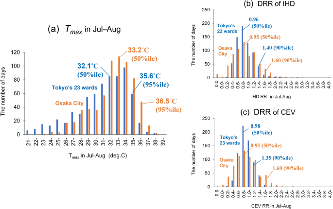
Figure 1 gives basic information on the daily maximum temperature (Tmax) and daily relative risk (DRR; normalised by yearly mean deaths in July–August) of IHD and CEV in July–August. The Tmax in Tokyo was approximately 1°C lower than that in Osaka at both of the 50th and 95th percentiles (Fig. 1a). While the DRRs of IHD and CEV at the 50th percentile were almost identical in Tokyo and Osaka, those at the 90th percentile in Tokyo were 1.14- to 1.19-fold lower than in Osaka (Fig. 1b,c). For example, the mortality of IHD and CEV in people of ages 65 + years in Tokyo accounted for 85.5% and 88.0% of the total in 2009–2019, of which 76.5% and 83.3% were in people of ages 75 + years. Hence, we additionally focused on people aged 65 + and 75 + years, because the risk for heat-related morbidity or mortality from cardiovascular diseases is higher in older people10.
Frequency of (a) Tmax, (b) DRR of IHD, and (c) DRR of CEV during 2009–2019 in Tokyo’s 23 wards and Osaka City. Tmax at the 50th and 95th percentiles and DRR at the 50th and 90th percentiles are shown in the respective graphs. Tmax daily maximum temperature, DRR daily relative risk, IHD ischaemic heart disease, CEV cerebrovascular disease.
Lag effect of weather exposure on mortality risk
The significance of delayed effects of daily weather conditions on mortality has been previously investigated using a distributed lag nonlinear model (DLNM)24 (see “Methods”). The results showed that the DRR of IHD increased rapidly with Tmax and daily mean water vapor pressure (Vap); Tmax and Vap exceeding 30 °C and 24 hPa, respectively, caused an exponential increase in IHD mortality risk in Tokyo (Fig. 2a,b; Fig. S2a–c for Osaka). In addition, the DRR remained higher with a higher Tmax or Vap delayed for > 1 week. Although the DRR of the IHD response to daily mean air pressure (Pres) was less sensitive than that to Tmax and Vap (Fig. 2c), the mortality risk persisted for > 10 days longer than those of Tmax and Vap, with a higher Pres.

Results of lag analysis using the DLNM in Tokyo. (a–c) DRR of IHD and (d–f) DRR of CEV for (a,d) Tmax, (b,e) Vap, and (c,f) Pres. Each panel indicates (left) weather variables versus DRR at lags of 0, 3, 6 days and (right) lag days versus DRR at the lower 5th, 50th, and upper 5th (95th) percentiles of weather variables. Tmax daily maximum temperature; Vap, daily mean water vapor pressure; Pres, daily mean air pressure; DLNM, distributed lag nonlinear model; DRR, daily relative risk; IHD, ischaemic heart disease; CEV, cerebrovascular disease.
The response of the CEV DRR to weather exposure was significantly weaker than that of IHD (Fig. 2d–f). However, the overall risk for CEV, which was integrated for all lag effects, was present for weather elements (Fig. S3).
Table 1 summarises the set of lag days used for the subsequent ML, based on the DLNM results. Here, lag days were specified for people aged all, aged 65 + years, and aged 75 + years (Fig. S4–S7 from DLNM results). If the lag effect on the mortality risk with weather exposure was longer than the maximum of 14 days used in the DLNM analyses, it was assigned as 14 days in the ML features. The existence of lag days suggests that weather features on previous days should be incorporated into ML (e.g., Tmax on the previous 1 day, 2 days, …, and 8 days for the DRR of IHD in Tokyo). Therefore, based on the data in Table 1, the Tmax, Vap, and Pres on previous days were added to the weather features used in ML implementation (Table 2).
Mortality hindcast with weather features
A mortality hindcast for 2009–2019 was performed using ML techniques with Boruta SHapley Additive exPlanations (BorutaSHAP)25 for feature selection (see “Methods”). A gradient boosting algorithm (LightGBM)26 was adopted as the ML method in this study (see “Methods”). The inputted initial features are listed in Table 2. The temperature-related features include Tmax on the day (Tmax), Tmax n days ago (TmaxPre n), the difference from n days ago (TmaxDiffPre n), and accumulated high temperature (AcTmax30) defined by:
Here, i represents the target date. Vapor- and air pressure-related features, daily rainfall, and the day of week were also used as initially inputted features (Table 2).
Figure 3 shows the results of ML and the selected features for Tokyo IHD mortality at all ages (Fig. S8a,b for ages 65 + years and 75 + years). In the BorutaSHAP analysis, Tmax, TmaxPre2, and AcTmax30 were selected from among the 37 features important for reproducing the DRR of IHD in Tokyo during the summer of each year (Fig. 3a-1). The model learning using these features related to temperature accurately reproduced the increases and decreases of the DRR in each year (Fig. 3a-2). Quantitative evaluation between the observed and simulated DRR yielded a root mean square error (RMSE) of 0.369, mean absolute error (MAE) of 0.290, and their ratio (RMSE/MAE) of 1.269.

ML hindcast of (a) IHD and (b) CEV mortality during summer in Tokyo (2009–2019). (1) Important features selected using BorutaSHAP, (2) comparison of the simulated and actual DRR, and (3) relationships between SHAP values and the selected important features. ML, machine learning; BorutaSHAP, Boruta SHapley Additive exPlanations; DRR, daily relative risk; IHD, ischaemic heart disease; CEV, cerebrovascular disease; RMSE, root mean square error; MAE, mean absolute error.
The daily instance of the SHAP26 value can explain the quantitative attribution of a selected feature. The positive values of SHAP, which indicate an increased DRR, increased rapidly when TmaxPre2 or Tmax exceeded approximately 34 °C (left and centre panels in Fig. 3a-3). However, an increase in AcTmax30 decreased the SHAP value (right panel in Fig. 3a-3), and the DRR of IHD was less likely to increase if AcTmax30 exceeded 130 °C. Meanwhile, ML implemented for Osaka selected only Tmax as an important feature for DRR, and the RMSE and MAE between the actual and simulated DRR were larger than those of Tokyo (Fig. S8c–e).
Optimal features for the DRR of CEV in Tokyo were not temperature-related features but rather air pressure-related PresDiffPre1 and PresPre14 (Fig. 3b-1). Although the reproduced DRR of CEV (Fig. 3b-2) indicated an RMSE of 0.326, MAE of 0.264, and RMSE/MAE of 1.236, which were nearly equivalent to those of the aforementioned IHD, the responses of SHAP to the two pressure-related features were less sensitive than those of IHD (Fig. 3b-3). The simulated DRR for people aged 65 + years was also not related to the selected features (Fig. S9a,b) whereas the ML for DRR of people aged 75 + years failed to select important features via BorutaSHAP. Hence, it was difficult to perform ML prediction of CEV mortality in association with weather changes in Tokyo and Osaka.
Future mortality risk
The sensitivity of IHD mortality risk to temperature-related features enabled estimation of changes in mortality risk caused by the hotter summers expected in the near future. Hence, the IHD mortality risk in Tokyo was evaluated with a sufficiently large population to avoid uncertainty. However, with a model trained using rare samples with a higher Tmax and higher DRR in the present era, it is difficult to predict unknown or little-experienced future warming influences on DRR. Therefore, we used a resampling architecture (see “Methods”), padding the rare samples to balance their appearance prior to executing ML, and transfer learning (TL) architecture (see “Methods”) for extrapolation from the past training data, in future risk estimations.
Figure 4 shows the effect of climate change over the next 20–30 years on Tokyo IHD mortality in people aged 75 + years (Fig. S10 for people aged 65 + years), which is expected to increase (Fig. S1). ML based on a model learned using the 2009–2019 dataset with the three important features (Tmax, TmaxPre2, and AcTmax30) was performed using future climate data for 2045–2055, predicted by the three global climate models: MRI-CGCM3 (Fig. 4a), MIROC5 (Fig. 4b), and GFDL-CM3 (Fig. 4c) under the RPC8.5 scenario from the NARO climate projection scenario dataset27 (see “Methods”). The temperatures predicted by the three models are known as the lowest (MRI-CGCM3), middle (MIROC5), and highest (GFDL-CM3) increasing tendencies from the present period (Fig. S10). Comparison with the DRR in 2009–2019 (the lower panels in Fig. 4) showed that each percentile of the estimated future DRR (approximately 30 years later) was higher than the present percentile for all of the climate models. The smallest increase in the future era was estimated to be 1.16-fold (1.04-fold) at the 95th percentile, corresponding to the upper 5% of overall days compared to the ML-simulated (actual) DRR at the present era, and 1.13-fold (0.97-fold) at the 99th percentile corresponding to the upper 1% of overall days. On the other hand, the largest increase was anticipated to be 1.29-fold (1.16-fold) at the 95th percentile and 1.35-fold (1.16-fold) at the 99th percentile compared to the ML-simulated (actual) DRR in the present era.

Frequency distributions (upper panels) and percentiles (lower panels) of the DRR of IHD for people aged 75 + years in Tokyo. Against actual and ML results in 2009–2019, the DRR change was estimated using climate projections of (a) MRI-CGCM3, (b) MIROC5, and (c) GFDL-CM3 under the RCP8.5 condition. “no TL” and “TL” indicate ML cases not incorporating TL and incorporating TL, respectively. ML machine learning, DRR daily relative risk, IHD ischaemic heart disease, TL transfer learning.
The effectiveness of TL using data of a hotter region (i.e., Osaka) in future warming projections for Tokyo is also indicated as “no TL” and “TL” in Fig. 4. Their comparison clarified that TL cases increased the DRR values relative to no TL cases in warmer climate models. This suggests that learning using high temperatures is needed for ML to perform well conditions of little experience with a future warmer climate in a target region (i.e., Tokyo). Incorporation of TL increased DRR by 2.2% and 7.5% at the 95th and 99th percentiles, respectively, compared to without TL, for the middle-level warming climate of MIROC5, and those increased DRR by 7.1% and 6.2% for the high-level warming climate of GFDL-CM3 (the lower panels in Fig. 4). Finally, ML incorporating TL showed that the daily IHD mortality risk in Tokyo on average increased by 29% and 35% at the 95th and 99th percentiles using the high-level warming climate scenario in 2045–2055, compared to the risk simulated using ML in 2009–2019.
Discussion
Pre-analyses using the DLNM suggested a requirement of lag-related weather elements for daily mortality when selecting features for inclusion in ML. Lag days of approximately 1 week for heat exposure (Tmax in this study) in IHD mortality (Fig. 2a–c) are supported by the results of a meta-analysis28 of research conducted in several countries. This 1-week delay of the mortality risk for IHD in summer is longer than that for heatstroke (0–2 days)29. The increase in cardiovascular disease mortality at higher temperatures is attributed to dehydration-induced increases in the viscosity of plasma, serum cholesterol levels, and red blood cell and platelet counts21,30. In addition, the increase in core body temperature caused by an exaggerated thermoregulatory response can lead to the development of acute cardiovascular diseases30.
Although CEV mortality is less sensitive to weather elements (Fig. 2d–f), the lag effect of Tmax and the longer-delayed effect of Pres were found to have weak responses in the DRR. In particular, pressure-related features tended to be selected as important features for the ML of CEV, instead of temperature-related features (Fig. 3b). A nonsignificant effect of high temperature on CEV mortality has been reported in several studies31. Although changes in pressure are related to CEV diseases, such as subarachnoid haemorrhage32, associations with air pressure in summer have not been epidemiologically confirmed. These characteristics of CEV hamper reproduction of the DRR with weather features using ML.
An additional temperature effect of AcTmax30 is likely needed to reproduce the DRR of IHD in Tokyo. Indeed, peaks in the DRR in 2018 and 2019 were reproduced by the inclusion of AcTmax30 when executing ML (Fig. S11). As suggested by the SHAP response to AcTmax30, an increase in AcTmax30 reduced the DRR of IHD (Fig. 3a-3), implying a kind of heat acclimatisation. Excessive heat loads to the human body have adverse effects on cardiovascular function (e.g., thermoregulatory disruption and haemoconcentration)33 whereas heat acclimatisation of the human body produces cardiovascular adaptation (improving physiological responses to heat)34, even with long-term heat exposure over several months35.
In this study, evaluations of future DRR possibilities using climate projection data were challenged for the IHD mortality risk in Tokyo. However, the influence of future further aging of the population on ML implementation was not considered. The DRR values defined in this study represent the relative mortality risks during summer of 1 year, to avoid the influence of year-to-year changes caused by, for example, natural progression of population aging and medical advances that extend longevity. However, the future DRR calculated for people aged 75 + years (Fig. 4) was probably underestimated in comparison with the actual DRR because of the growth of the population older people aged 85 + years.
TL has been applied to predict future change in various disciplines, such as Earth sciences36,37,38. In this study, we evaluated the change in mortality risk under future climate conditions, incorporating TL and imbalanced learning (or resampling)39,40 architectures. A similar method has been used to forecast extreme heatwaves41. Because the characteristics that related Tmax to DRR in Osaka City (“source or supporting data” in TL) except for population size were similar to those in Tokyo’s 23 wards (“target data” in TL) (Fig. 1), ML implementation with TL was effective for higher-level climate warming (predicted by MIROC5 and GFDL-CM3) in Tokyo.
Because evaluation of the future mortality from ML and applying TL is breakthrough challenging, it is difficult to ensure the accuracy of the predicted mortality risk. However, use of the actual relationships between mortality risk and weather conditions in Osaka City, which are not currently experienced in Tokyo, can interpolatively predict a potential future mortality risk in Tokyo. TL was conducted using artificial data over-sampled around the upper 10% of the DRR in Tokyo, which was rare from 2009 to 2019. This resampling technique increased the DRR at the maximum frequency of appearance by 1.3-fold. Future deaths owing to IHD in Tokyo have not been officially analysed, whereas it is estimated that the number of inpatients with cardiovascular diseases will increase 1.3-fold by 2050 compared to 201518. Hence, over-sampling at the upper 10% of DRR should be used in future investigations.
Methods
Daily weather data
Agro-Meteorological Grid Square Data (https://amu.rd.naro.go.jp/) provided by the National Agriculture and Food Research Organization (NARO)42 were used to assess daily weather conditions in Tokyo and Osaka. These data were developed by 1 km spatial interpolation of meteorological elements (e.g., temperature, wind speed, rainfall, and solar radiation) measured nationwide in Japan at observation stations of the Japan Meteorological Agency (JMA). Temperature-related data were corrected for grid altitude. In this study, Tmax (°C) and Rain (mm) were extracted and averaged for grids corresponding to Tokyo’s 23 wards (986 grids) and Osaka City (422 grids), as shown in Fig. 5. Pres and Vap data were from the JMA observation station (https://www.jma.go.jp) located in the centre of Tokyo and Osaka, because the abovementioned Agro-Meteorological Grid Square Data do not include those elements.

Weather data grids (red dots in maps at left) and summer ischaemic heart disease (IHD) and cerebrovascular disease (CEV) mortality rates according to age group (pie charts at right) analysed in (a) Tokyo and (b) Osaka. Gridded weather data at 1 km resolution from the Agro-Meteorological Grid Square Data provided by the NARO were used. Mortality data were extracted for July–August from 2009 to 2019. The Generic Mapping Tools (GMT) graphic system (version 6.4.0; https://www.generic-mapping-tools.org/team.html) was used to draw the maps.
Daily mortality data
Statistical surveillance information regarding the number of daily deaths (https://www.e-stat.go.jp/en) published by the Ministry of Health, Labour and Welfare (MHLW) of the Japanese government were used in this study. Information such as the cause of death, age, and sex was included in the data. The International Statistical Classification of Diseases and Related Health Problems 10th Revision (ICD-10) was used to classify causes of death. We analysed the following I20–25 and I60–63 codes corresponding to IHD and CEV, respectively: I20, angina pectoris; I21, acute myocardial infarction; I22, subsequent myocardial infarction; I23, certain current complications following acute myocardial infarction; I24, other acute ischaemic heart diseases; I25, chronic ischaemic heart disease; I60, subarachnoid haemorrhage (including sequelae, I69.0); I61, intracerebral haemorrhage (including sequelae, I69.1); I62, other nontraumatic intracranial haemorrhage (including sequelae, I69.2); and I63, cerebral infarction (including sequelae, I69.3). The mortality from IHD and CEV was approximately 60–70% in people aged 75 + years (Fig. 5).
Lag analysis and machine learning
Figure 6 depicts the flow of analysis in this study. We conducted: (A) a lag analysis for feature selection related to IHD or CEV mortality, (B) pre-analyses for ML, and (C) mortality hindcast and future risk evaluation using ML.

Flow of analysis in this study. We performed “lag analysis for feature selection”, “pre-analyses for machine learning”, and “machine learning performance”. DLNM, distributed lag nonlinear model; SHAP, SHapley Additive exPlanations; GBDT, gradient boosting decision tree.
Lag analysis
The DLNM24 was used to reveal a delayed weather effect on IHD and CEV mortality in the part (A) of Fig. 6. This model has been used in public health studies43 and is defined using the following model equation:
Here, NDt represents the expected number of deaths at day t in which the error function was assumed to follow a quasi-Poisson distribution. cbt,l is the cross-basis matrix for a weather variable (Tmax, Vap, or Pres) with t and lag days l, which is produced by the DLNM fitting the nonlinear and lag effects. ns means a natural spline function, which was examined for the date with the degree of freedom per year (df = 2) and year = 11. This term works to adjust long-term trends. However, the influence of day of the week on mortality was negligible according to sensitivity experiments including or excluding the term in Eq. (2). The exposure–response curves were modelled by a natural cubic function with 2 degrees of freedom for variables and lag days. Those knots were placed at equally-spaced values in the temperature range and at equal intervals on a logarithmic scale for lag days by default24.
The maximum number of lag days was assigned as 14 days (2 weeks), and two degrees of freedom were used for the weather variable and lag effect. Moghadamnia et al.28 revealed that temperature lag affected the risk for cardiovascular mortality year-round with the greatest risk at 14 lag days, by their systematic review and meta-analysis worldwide. Because heat-related mortality indicates shorter lag effects than cold-related mortality, we set 14 days as the maximum lag days. In addition, we assumed identical maximum lag effects of weather parameters other than temperature because lag effects on mortality risk have not been revealed.
The DLNM was conducted for one of the three weather variables (i.e., Tmax, Vap, or Pres) without incorporating the other two variables as confounders, because the specified lag days for selecting ML features were unaffected even if confounders were incorporated to implementations of DLNM.
Feature selection
BorutaSHAP25, which combines the Boruta feature selection algorithm with SHAP, was also used in part (B) of Fig. 6. The Boruta feature selection is a wrapper method for detecting important features in ML44,45: Shuffled duplicates (shadow features as noise) of all features are added as unpredictability to the original feature dataset (e.g., Tmax, TmaxPre2, …, Pres, PresPre2, …); next, feature importance based on Z-scores in the enlarged dataset (i.e., original features + shadow features) is used to train a decision tree-based algorithm (Gradient Boosting Decision Trees in this study). Each training cycle is analysed for a higher priority feature than the most important shadow feature, and elements considered highly irrelevant are deleted.
BorutaSHAP provides flexibility in model selection and allows visualisation of the selected features by applying the SHAP25. The SHAP, i.e., “Shapley value,” has been originally developed to estimate the contribution of an individual player in a collaborative team and ensure fair allocation according to their contribution46,47. Features (daily weather elements in this study) contribute to the model’s output or prediction with a different magnitude (importance) and sign (positive or negative), which is accounted for by the Shapley values48.
Machine learning (ML)
A gradient boosting algorithm was adopted as the ML used in part (C) of Fig. 6; this is an ensemble learning technique to improve the performance of ML49,50. Ensemble learning includes multiple models termed “weak learners” (generally decision trees); their outputs are combined for prediction or classification problems25. Boosting learners learn in a sequential manner to correct errors from the previous learner and create a robust model to reduce model bias. Therefore, a gradient boosting ML increases accuracy more than other ML algorithms, such as random forest49,51. In this study, the LightGBM26 was adopted as a gradient boosting ML, which significantly outperforms other gradient boosting algorithms in terms of computational speed and memory consumption52.
The 2009–2019 dataset was divided into 10 groups and iteratively evaluated using a k-fold cross-validation method53 (i.e., k = 10), which used 90% of the data as training data and the remaining 10% as testing data. In searching the best hyperparameters in the ML model, “the number of leaves” parameter required for leaf-wise tree growth, which is adopted in LightGBM, was optimised from values of 10–100 for ML.
Evaluation to future climate change
Transfer learning (TL)
A TL architecture54,55,56 was applied to evaluate future mortality in this study. Because the present era (2009–2019) data did not include many days with higher temperature which could happen frequently in the future climate, the future DRR evaluated by ML may be biased toward the present average temperatures. Therefore, to resample the present (2009–2019) data to the higher frequency of high-temperature appearance days in the future, the Synthetic Minority Over-Sampling Technique for Regression with Gaussian Noise (SMOGN)57 was implemented as a pre-processor for TL. Regression analysis often targets an accurate prediction of rarely occurring extreme values of an objective variable, which is assigned continuous values. To increase the frequency of rare instances (days with extremely high temperatures in this study), imaginary data were generated by applying Gaussian noise to the rare samples. Resamples using the SMOGN were adjusted to be over-sampled around the upper 10% of DRR in Tokyo, which is rare in the present era but could be more frequent in the future.
TL was applied to explore future possibilities for DRR of IHD in Tokyo, which can improve the prediction accuracy of a task for a target domain (Tokyo data) in conjunction with information obtained from a task for a source domain (Osaka data). This situation corresponds to a simple “homogeneous transfer” with transformation of the source domain to the target domain. If there is an available dataset drawn from a domain related to but not exactly matching a target domain of interest, homogeneous TL can be used to build a predictive model for the target domain as long as the input feature space is the same55. A feature-based algorithm of the Feature Augmentation Method58 was adopted as TL to evaluate changes in risk. The augmented source data contain common and source-specific domains, whereas the augmented target data contain common and target-specific domains. Hence, the feature dimension is augmented threefold ((chi to overset{lower0.5emhbox{$smash{scriptscriptstylesmile}$}}{chi }) (={mathbb{R}}^{3F}); χ denotes a feature domain, (overset{lower0.5emhbox{$smash{scriptscriptstylesmile}$}}{chi }) an augmented feature domain, and ({mathbb{R}}^{3F}) a three-dimensional real space). Next, it is defined as Φs and Φt as mappings of the source and target data, respectively, for (chi to overset{lower0.5emhbox{$smash{scriptscriptstylesmile}$}}{chi }):
Here, 0 is the zero vector and x is the feature vector of the source or target domain. Finally, supervised learning was implemented by assigning the dataset of Tokyo as Φt and that of Osaka as Φs.
Climate change projection
The Regional Climate Projection Scenario Dataset27 (https://amu.rd.naro.go.jp/) provided by the NARO was used to evaluate the effect of future climate change on the DRR of IHD in Tokyo. The output results, simulated using several global climate models, were statistically downscaled to the Japanese regional model with 1 km spatial resolution. A Gaussian-type scaling approach59 was adopted as a statistical downscaling method to improve the reproducibility of daily and annual variation. Based on the relationship between the standard deviations (e.g., temperature, wind speed, rainfall, and solar radiation) of the global climate model and observations for a past reference period, means and standard deviations were corrected such that the climate change signal would not be enhanced60.
From published output results of several models, the MRI-CGCM3 (Japan; Meteorological Research Institute), MIROC5 (Japan; The University of Tokyo, National Institute for Environmental Studies, and Japan Agency for Marine–Earth Science and Technology), and GFDL-CM3 (USA; NOAA Geophysical Fluid Dynamics Laboratory) models, which were used in the Coupled Model Intercomparison Project phase 5 (CMIP5)61, were chosen because the simulated temperature bias included low, middle, and high levels, respectively, of the NARO climate projection scenario dataset62 (cf. Fig. S12). In addition, these model projections included the two scenarios RCP2.6 (low-emissions scenario via stringent mitigation) and RCP8.5 (high-emissions scenario without any mitigation) of the greenhouse gas emissions “pathway”63. In this study, we used the projection result of RCP8.5 as the worst-case climate scenario to evaluate the future IHD risk.
Data availability
The data that support the findings of this study are available from the NARO portal site of official statistics published (gridded weather and climate scenario data; https://amu.rd.naro.go.jp/) and MHLW (death data; https://www.e-stat.go.jp/en). These data are of restricted availability, and we used them with permission for this study. Therefore, data are available from the corresponding author upon reasonable request and with the permission of the NARO and the MHLW.
References
-
Revich, B. & Shaposhnikov, D. The influence of heat and cold waves on mortality in Russian subarctic cities with varying climates. Int. J. Biometeorol. 66, 2501–2515. https://doi.org/10.1007/s00484-022-02375-2 (2022).
Google Scholar
-
Petkova, E. P., Dimitrova, L. K., Sera, F. & Gasparrini, A. Mortality attributable to heat and cold among the elderly in Sofia, Bulgaria. Int. J. Biometeorol. 65, 865–872. https://doi.org/10.1007/s00484-020-02064-y (2021).
Google Scholar
-
Son, J.-Y., Gouveia, N., Bravo, M. A., de Freitas, C. U. & Bell, M. L. The impact of temperature on mortality in a subtropical city: Effects of cold, heat, and heat waves in São Paulo, Brazil. Int. J. Biometeorol. 60, 113–121. https://doi.org/10.1007/s00484-015-1009-7 (2016).
Google Scholar
-
Tan, J. et al. The urban heat island and its impact on heat waves and human health in Shanghai. Int. J. Biometeorol. 54, 75–84. https://doi.org/10.1007/s00484-009-0256-x (2010).
Google Scholar
-
Takahashi, K., Honda, Y. & Emori, S. Assessing mortality risk from heat stress due to global warming. J. Risk Res. 10, 339–354. https://doi.org/10.1080/13669870701217375 (2007).
Google Scholar
-
Zeppetello, L. R. V., Raftery, A. E. & Battisti, D. S. Probabilistic projections of increased heat stress driven by climate change. Commun. Earth Environ. 3, 183. https://doi.org/10.1038/s43247-022-00524-4 (2022).
Google Scholar
-
Liu, L. et al. Associations between air temperature and cardio-respiratory mortality in the urban area of Beijing, China: A time-series analysis. Environ. Health. 10, 51. https://doi.org/10.1186/1476-069X-10-51 (2011).
Google Scholar
-
de Blois, J. et al. The effects of climate change on cardiac health. Cardiology 131, 209–217. https://doi.org/10.1159/000398787 (2015).
Google Scholar
-
Achebak, H., Devolder, D., Ingole, V. & Ballester, J. Reversal of the seasonality of temperature-attributable mortality from respiratory diseases in Spain. Nat. Commun. 11, 2457. https://doi.org/10.1038/s41467-020-16273-x (2020).
Google Scholar
-
Bunker, A. et al. Effects of air temperature on climate-sensitive mortality and morbidity outcomes in the elderly: A systematic review and meta-analysis of epidemiological evidence. EBioMedicine 6, 258–268. https://doi.org/10.1016/j.ebiom.2016.02.034 (2016).
Google Scholar
-
World Health Organisation. Cardiovascular Diseases (CVDs). https://www.who.int/news-room/fact-sheets/detail/cardiovascular-diseases-(cvds) (2021).
-
Wlodarczyk, A. et al. Machine learning analyzed weather conditions as an effective means in the predicting of acute coronary syndrome prevalence. Front. Cardiovasc. Med. 9, 830823. https://doi.org/10.3389/fcvm.2022.830823 (2022).
Google Scholar
-
Matheson, M. B. et al. Cardiovascular risk prediction using machine learning in a large Japanese cohort. Circ. Rep. 4, 595–603. https://doi.org/10.1253/circrep.CR-22-0101 (2022).
Google Scholar
-
Lin, Y.-C., Tsai, C.-H., Hsu, H.-T. & Lin, C.-H. Using machine learning to analyze and predict the relations between cardiovascular disease incidence, extreme temperature and air pollution. 2021 IEEE 3rd Eurasia Conference on Biomedical Engineering, Healthcare and Sustainability (ECBIOS) 234–237. https://doi.org/10.1109/ECBIOS51820.2021.9510479 (2021).
-
Lee, W., Lim, Y. H., Ha, E., Kim, Y. & Lee, W. K. Forecasting of non-accidental, cardiovascular, and respiratory mortality with environmental exposures adopting machine learning approaches. Environ. Sci. Pollut. Res. 29, 88318–88329. https://doi.org/10.1007/s11356-022-21768-9 (2022).
Google Scholar
-
Cabinet Office, Government of Japan. Aging Population (in Japanese). https://www8.cao.go.jp/kourei/whitepaper/w-2020/html/zenbun/s1_1_1.html (2022).
-
Ministry of Health, Labour and Welfare, Government of Japan. Vital Statistics in 2019 (in Japanese). https://www.mhlw.go.jp/toukei/saikin/hw/jinkou/geppo/nengai19/dl/gaikyouR1.pdf (2020).
-
Ministry of Health, Labour and Welfare, Government of Japan. Estimation of Future Inpatients (in Japanese). https://www.mhlw.go.jp/file/05-Shingikai-12404000-Hokenkyoku-Iryouka/0000155222.pdf (2017).
-
Hirano, Y. et al. Machine learning-based mortality prediction model for heat-related illness. Sci. Rep. 11, 9501. https://doi.org/10.1038/s41598-021-88581-1 (2021).
Google Scholar
-
Ogata, S. et al. Heatstroke predictions by machine learning, weather information, and an all-population registry for 12-hour heatstroke alerts. Nat. Commun. 12, 4575. https://doi.org/10.1038/s41467-021-24823-0 (2021).
Google Scholar
-
Ohashi, Y., Miyata, A. & Ihara, T. Mortality sensitivity of cardiovascular, cerebrovascular, and respiratory diseases to warm season climate in Japanese cities. Atmosphere 12, 1546. https://doi.org/10.3390/atmos12121546 (2021).
Google Scholar
-
Yang, J. et al. Cardiovascular mortality risk attributable to ambient temperature in China. Heart 101, 1966–1972. https://doi.org/10.1136/heartjnl-2015-308062 (2015).
Google Scholar
-
Lim, Y.-H., Park, M.-S., Kim, Y., Kim, H. & Hong, Y.-C. Effects of cold and hot temperature dehydration: A mechanism of cardiovascular burden. Int. J. Biometeorol. 59, 1035–1043. https://doi.org/10.1007/s00484-014-0917-2 (2015).
Google Scholar
-
Gasparrini, A., Armstrong, B. & Kenward, M. G. Distributed lag non-linear models. Stat. Med. 29, 2224–2234. https://doi.org/10.1002/sim.3940 (2010).
Google Scholar
-
Eoghan, K. BorutaShap: A Wrapper Feature Selection Method Which Combines the Boruta Feature Selection Algorithm with Shapley Values. https://zenodo.org/record/4247618 (2020).
-
Lundberg, S. M. & Lee, S.-I. A unified approach to interpreting model predictions. Proceedings of the 31st International Conference on Neural Information Processing Systems 4768–4777 (2017).
-
Nishimori, M., Ishigooka, Y., Kuwagata, T., Takimoto, T. & Endo, N. SI-CAT 1km-grid square regional climate projection scenario dataset for agricultural use (NARO2017) (in Japanese). J. Jpn. Soc. Simul. Technol. 38, 150–154 (2019).
-
Moghadamnia, M. T. et al. Ambient temperature and cardiovascular mortality: A systematic review and meta-analysis. PeerJ. 5, e3574. https://doi.org/10.7717/peerj.3574 (2017).
Google Scholar
-
Oka, K., Honda, Y., Phung, V. L. H. & Hijioka, Y. Potential effect of heat adaptation on association between number of heatstroke patients transported by ambulance and wet bulb globe temperature in Japan. Environ. Res. 216, 114666. https://doi.org/10.1016/j.envres.2022.114666 (2023).
Google Scholar
-
Alahmad, B. et al. Cardiovascular mortality and exposure to heat an inherently hot region: Implications for climate change. Circulation 141, 1271–1273. https://doi.org/10.1161/CIRCULATIONAHA.119.044860 (2020).
Google Scholar
-
Zhang, Y. et al. The effects of ambient temperature on cerebrovascular mortality: An epidemiologic study in four climatic zones in China. Environ. Health 13, 24. https://doi.org/10.1186/1476-069X-13-24 (2014).
Google Scholar
-
Landers, A. T., Narotami, P. K., Govender, S. T. & Van Dellen, J. R. The effect of changes in barometric pressure on the risk of rupture of intracranial aneurysms. Br. J. Neurosurg. 11, 1919–2195. https://doi.org/10.1080/02688699746230 (1997).
Google Scholar
-
Donaldson, G. C., Keatinge, W. R. & Saunders, R. D. Cardiovascular responses to heat stress and their adverse consequences in healthy and vulnerable human populations. Int. J. Hyperth. 19, 225–235. https://doi.org/10.1080/0265673021000058357 (2003).
Google Scholar
-
Gibson, O. R., Taylor, L., Watt, P. W. & Maxwell, N. S. Cross-adaptation: Heat and cold adaptation to improve physiological and cellular responses to hypoxia. Sports Med. 47, 1751–1768. https://doi.org/10.1007/s40279-017-0717-z (2017).
Google Scholar
-
Malgoyre, A. et al. Four-month operational heat acclimatization positively affects the level of heat tolerance 6 months later. Sci. Rep. 10, 20260. https://doi.org/10.1038/s41598-020-77358-7 (2020).
Google Scholar
-
Zhao, Y. et al. Transfer-learning-based approach for yield prediction of winter wheat from planet data and SAFY Model. Remote Sens. 14, 5474. https://doi.org/10.3390/rs14215474 (2022).
Google Scholar
-
Wang, K., Johnson, C. W., Bennett, K. C. & Johnson, P. A. Predicting fault slip via transfer learning. Nat. Commun. 12, 7319. https://doi.org/10.1038/s41467-021-27553-5 (2021).
Google Scholar
-
Li, Q. et al. Improved daily SMAP satellite soil moisture prediction over China using deep learning model with transfer learning. J. Hydrol. 600, 126698. https://doi.org/10.1016/j.jhydrol.2021.126698 (2021).
Google Scholar
-
Japkowicz, N. & Stephen, S. The class imbalance problem: A systematic study. Intell. Data Anal. 6, 429–449. https://doi.org/10.3233/IDA-2002-6504 (2002).
Google Scholar
-
Krawczyk, B. Learning from imbalanced data: Open challenges and future directions. Prog. Artif. Intell. 5, 221–232. https://doi.org/10.1007/s13748-016-0094-0 (2016).
Google Scholar
-
Jacques-Dumas, V., Ragone, F., Borgnat, P., Abry, P. & Bouchet, F. Deep learning-based extreme heatwave forecast. Front. Clim. 4, 789641. https://doi.org/10.3389/fclim.2022.789641 (2022).
Google Scholar
-
Ohno, H., Sasaki, K., Ohara, G. & Nakazono, K. Development of grid square air temperature and precipitation data compiled from observed, forecasted, and climatic normal data. Clim. Biosphere 16, 71–79. https://doi.org/10.2480/cib.J-16-028 (2016).
Google Scholar
-
Sahani, J., Kumar, P., Debele, S. & Emmanuel, R. Heat risk of mortality in two different regions of the United Kingdom. Sustain. Cities Soc. 80, 103758. https://doi.org/10.1016/j.scs.2022.103758 (2022).
Google Scholar
-
Kim, J., Lee, J. & Park, M. Identification of smartwatch-collected lifelog variables affecting body mass index in middle-aged people using regression machine learning algorithms and SHapley Additive Explanations. Appl. Sci. 12, 3819. https://doi.org/10.3390/app12083819 (2022).
Google Scholar
-
Wu, J., Orlandi, F., O’Sullivan, D., Pisoni, E. & Dev, S. Boosting climate analysis with semantically uplifted knowledge graphs. IEEE J Sel. Top. Appl. Earth Obs. Remote Sens. 15, 4708–4718. https://doi.org/10.1109/JSTARS.2022.3177463 (2022).
Google Scholar
-
Rodríguez-Pérez, R. & Bajorath, J. Interpretation of machine learning models using shapley values: Application to compound potency and multi-target activity predictions. J. Comput. Aided Mol. Des. 34, 1013–1026. https://doi.org/10.1007/s10822-020-00314-0 (2020).
Google Scholar
-
Nohara, Y., Matsumoto, K., Soejima, H. & Nakashima, N. Explanation of machine learning models using shapley additive explanation and application for real data in hospital. Comput. Methods Progr. Biomed. 214, 106584. https://doi.org/10.1016/j.cmpb.2021.106584 (2022).
Google Scholar
-
Mosca, E., Szigeti, F., Tragianni, S., Gallagher, D. & Groh, G. SHAP-based explanation methods: a review for NLP interpretability. In Proceedings of the 29th International Conference on Computational Linguistics 4593–4603 (International Committee on Computational Linguistics, 2022).
-
Natekin, A. & Knoll, A. Gradient boosting machines, a tutorial. Front. Neurorobot. 7, 21. https://doi.org/10.3389/fnbot.2013.00021 (2013).
Google Scholar
-
Sibindi, R., Mwangi, R. W. & Waititu, A. G. A boosting ensemble learning based hybrid light gradient boosting machine and extreme gradient boosting model for predicting house prices. Eng. Rep. 5, e12599. https://doi.org/10.1002/eng2.12599 (2022).
Google Scholar
-
Ghazwani, M. & Begum, M. Y. Computational intelligence modeling of hyoscine drug solubility and solvent density in supercritical processing: Gradient boosting, extra trees, and random forest models. Sci. Rep. 13, 10046. https://doi.org/10.1038/s41598-023-37232-8 (2023).
Google Scholar
-
Zhou, Z.H. Ensemble learning. In: Li, S.Z., Jain, A. (eds) Encyclopedia of Biometrics. Springer, Boston, MA. (2009).
-
Burman, P. A comparative study of ordinary cross-validation, v-fold cross-validation and the repeated learning-testing methods. Biometrika 76, 503–514. https://doi.org/10.2307/2336116 (1989).
Google Scholar
-
Hosna, A. et al. Transfer learning: A friendly introduction. J. Big Data 9, 102. https://doi.org/10.1186/s40537-022-00652-w (2022).
Google Scholar
-
Weiss, K., Khoshgoftaar, T. M. & Wang, D. A survey of transfer learning. J. Big Data 3, 9. https://doi.org/10.1186/s40537-016-0043-6 (2016).
Google Scholar
-
Obst, D. et al. Improved linear regression prediction by transfer learning. Comput. Stat. Data Anal. 174, 107499. https://doi.org/10.1016/j.csda.2022.107499 (2022).
Google Scholar
-
Branco, P., Torgo, L. & Ribeiro, R. P. SMOGN: A pre-processing approach for imbalanced regression. Proc. Mach. Learn. Res. 74, 36–50 (2017).
-
Daumé, H. III. Frustratingly easy domain adaptation. Proceedings of the 45th Annual Meeting of the Association of Computational Linguistics 256–263 (2007).
-
Haerter, J. O., Hagemann, S., Moseley, C. & Piani, C. Climate model bias correction and the role of timescales. Hydrol. Earth Syst. Sci. 15, 1065–1079. https://doi.org/10.5194/hess-15-1065-2011 (2011).
Google Scholar
-
Ishizaki, N. N. et al. Evaluation of two bias-correction methods for gridded climate scenarios over Japan. SOLA 16, 80–85. https://doi.org/10.2151/sola.2020-014 (2020).
Google Scholar
-
Taylor, K. E., Stouffer, R. J. & Meehl, G. A. An overview of CMIP5 and the experiment design. Bull. Am. Meteorol. Soc. 93, 485–498. https://doi.org/10.1175/BAMS-D-11-00094.1 (2012).
Google Scholar
-
The NARO. Standard Operating Procedures for the Use of the Regional Climate Scenario Dataset for the Assessment of Regional Climate Change Adaptation Measures (Public Version in Japanese). https://www.naro.go.jp/publicity_report/publication/files/SOP20-402K20210916.pdf (2021).
-
IPCC AR5 Synthesis Report: Climate Change 2014. https://www.ipcc.ch/report/ar5/syr/ (2014).
Acknowledgements
The mortality data were provided by the MHLW of the Japanese Government through official procedures. The authors thank Dr. Yasushi Honda (National Institute for Environmental Studies, Japan) for advice on our analyses.
Funding
The Funding was provided by Japan Society for the Promotion of Science (Grant Number: 20H03949).
Author information
Authors and Affiliations
Contributions
Study concept and design: Y.O. Data acquisition: Y.O., T.I., and Y.T. Analysis and interpretation of data: Y.O., T.I, and K.O. Drafting of the manuscript: Y.O. Discussion and revision of the manuscript: all authors. All authors reviewed the final manuscript.
Corresponding author
Ethics declarations
Competing interests
The authors declare no competing interests.
Additional information
Publisher’s note
Springer Nature remains neutral with regard to jurisdictional claims in published maps and institutional affiliations.
Supplementary Information
Supplementary Information.
Rights and permissions
Open Access This article is licensed under a Creative Commons Attribution 4.0 International License, which permits use, sharing, adaptation, distribution and reproduction in any medium or format, as long as you give appropriate credit to the original author(s) and the source, provide a link to the Creative Commons licence, and indicate if changes were made. The images or other third party material in this article are included in the article’s Creative Commons licence, unless indicated otherwise in a credit line to the material. If material is not included in the article’s Creative Commons licence and your intended use is not permitted by statutory regulation or exceeds the permitted use, you will need to obtain permission directly from the copyright holder. To view a copy of this licence, visit http://creativecommons.org/licenses/by/4.0/.
Reprints and Permissions
About this article
Cite this article
Ohashi, Y., Ihara, T., Oka, K. et al. Machine learning analysis and risk prediction of weather-sensitive mortality related to cardiovascular disease during summer in Tokyo, Japan.
Sci Rep 13, 17020 (2023). https://doi.org/10.1038/s41598-023-44181-9
-
Received: 28 March 2023
-
Accepted: 04 October 2023
-
Published: 09 October 2023
-
DOI: https://doi.org/10.1038/s41598-023-44181-9
Comments
By submitting a comment you agree to abide by our Terms and Community Guidelines. If you find something abusive or that does not comply with our terms or guidelines please flag it as inappropriate.